Coin Tossing and Family Size

If you a toss a coin 9 times, what is the probability of obtaining 8 heads and 1 tail? I just tossed one penny 9 times and the following is the resulting sequence of heads and tails.

. \ \ \ \ \ \ \ \ T \ T \ H \ T \ H \ H \ H \ T \ H

The above little experiment produced 5 heads and 4 tails, matching what many people think should happen when you toss a coin repeatedly, i.e., roughly half of the tosses are heads and half of the tosses are tails. Does this mean that it is impossible to get 8 heads in 9 tosses? It turns out that it is possible, just that such scenarios do not happen very often. On average, you will have to do the 9-toss experiments many times before you will see a result such as H \ H \ H \ T \ H \ H \ H \ H \ H. The coin tossing example is a great way to introduce the binomial distribution.

One concrete example of 8 heads in 9 tosses is the family of Olive and George Osmond. They are the parents of nine children, 8 boys and 1 girl, seven of which formed a popular and successful family singing group called The Osmond Brothers. Two of its members, Donny and Marie Osmonds, also had successful solo musical careers. Donny and Marie were both teen idols in the 1970s. The first picture below is a picture of Donny and Marie Osmond in their heyday. The second picture is a photo of seven of the Osmond siblings who are in show business.


Donny and Marie Osmond in their heyday


Seven of the Osmond siblings who are in show business

Assuming that a boy is equally likely as a girl in a pregnancy, the sex of a child is like a coin toss (from a probability point of view). So the Osmond family shows that tossing a coin 9 times can result in 8 heads. But how often does this happen? Of all the families with 9 children, how many of them have 8 boys and 1 girl?

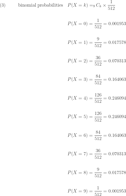
We will show that the probability of obtaining 8 heads in 9 tosses is 0.0176. This means that in 10,000 tosses of a coin, only 176 of the tosses have 8 heads and 1 tail. Looking at this from a family perspective, out of 10,000 families with 9 children, only about 176 have 8 boys and 1 girl (1.76%). So families such as the Osmond family are pretty rare.

The Problem

The problem we want to work on is this:

  • In tossing a fair coin 9 times, what is the probability that there are k heads? Here, k can be any whole number from 0 to 9.

For convenience, we use X to denote the number of heads that appear as a result of tossing a coin 9 times. We are interested in knowing the probability that X=k (k can be any whole number from 0 to 9). We use the notation P(X=k) to denote this probability. In the subsequent discussion, we derive P(X=k) for each value of k.

Two important things about this problem. One is that there are 2^9=512 many outcomes in tossing a coin 9 times. To see this, there are 2 outcomes in tossing a coin 1 time (H or T). There are 4 outcomes in tossing a coin 2 times (HH, HT, TH, and TT). So the number of outcomes in a coin tossing experiment is 2 raised to the number of tosses. For convenience, we denote each outcome by the string of Hs and Ts in the order the heads (Hs) and tails (Ts) appear. The following are four examples of such strings:

. \ \ \ \ \ \ \ \ T \ T \ T \ T \ T \ T \ T \ T \ T

. \ \ \ \ \ \ \ \ T \ T \ H \ T \ T \ T \ T \ T \ T

. \ \ \ \ \ \ \ \ H \ T \ H \ T \ T \ T \ T \ T \ T

. \ \ \ \ \ \ \ \ T \ T \ H \ T \ H \ H \ T \ T \ T

The second important thing is that each of the 512 strings has a probability of \frac{1}{512} since we are using a fair coin. In any toss, the probability of a head is \frac{1}{2}. So the problem of finding P(X=k) is to count how many of the 512 strings have k Hs and 9-k Ts. In other words, the problem at hand is that of a counting problem (or a combinatorial problem).

For example, there are nine strings consisting of 8 Hs and 1 T (the one T can be in any one of the nine positions). So we have:

\displaystyle . \ \ \ \ \ \ \ \ P(X=\text{8})=9 \times \frac{1}{512}=\frac{9}{512}=0.0176

The following is how we find the probability P(X=k):

\displaystyle . \ \ \ \ \ \ \ \ P(X=k) = \text{(the number of strings with k Hs)} \times \frac{1}{512}

To find P(X=0), we need to find the number of strings with zero H. There is only one (all nine positions are T). So we have:

\displaystyle . \ \ \ \ \ \ \ \ P(X=0)=1 \times \frac{1}{512}=\frac{1}{512}=0.001953

To find P(X=1), we need to count the number of strings with exactly 1 H. There are 9 such strings since the one H can be in any one of the nine positions. So we have:

\displaystyle . \ \ \ \ \ \ \ \ P(X=1)=9 \times \frac{1}{512}=\frac{9}{512}=0.0176

To find P(X=2), we need to count the number of strings with exactly 2 Hs in the nine positions. Here is where we need to formula to help us do the counting.

The Binomial Coefficient

We need a combinatorial formula to help us count the number of the letter H in a string of 9 letters of H and T. How many of the 512 strings have 2 Hs and 7 Ts? There are 36 (HHTTTTTTT, and HTHTTTTTT are two such strings). The calculation is:

\displaystyle (1) \ \ \ \ \ \ \ \ \frac{9!}{2! \times (9-2)!}=\frac{9!}{2! \times 7!}=\frac{9 \times 8}{2}=36

The above calculation uses the factorial notation:

. \ \ \ \ \ \ \ \ n!= n \times (n-1) \times (n-2) \times \cdots \times 3 \times 2 \times 1

In addition, we define 0!=1. More about the formula (1) later. For now we can calculate P(X=2):

\displaystyle . \ \ \ \ \ \ \ \ P(X=2)=36 \times \frac{1}{512}=\frac{36}{512}=0.070313

Suppose we have n positions and each position is H or T. There should be 2^n many strings consisting of Hs and Ts. The general formula is called the Binomial Coefficient, which is to count the number of strings with r Hs and n-r Ts.

\displaystyle (2) \ \ \ \ \ \ \ \ _nC_r = \frac{n!}{r! \times (n-r)!} \ \ \ \ \ \ \ \ \ \ \ \ \ \  \text{Binomial Coefficient}

Plugging into the formula, we have _9C_3=84, and _9C_4=126. So of the 512 strings consisting of Hs and Ts, 84 of them have 3 Hs and 6 Ts, and 126 of them have 4 Hs and 5 Ts. We have the following probabilities:

\displaystyle \begin{aligned}(3) \ \ \ \ \ \ \ \ \text{binomial probabilities} \ \ \ &P(X=k)=_9C_k \times \frac{1}{512} \\&\text{ } \\&P(X=0)=\frac{1}{512}=0.001953 \\&\text{ } \\&P(X=1)=\frac{9}{512}=0.017578 \\&\text{ } \\&P(X=2)=\frac{36}{512}=0.070313 \\&\text{ } \\&P(X=3)=\frac{84}{512}=0.164063 \\&\text{ } \\&P(X=4)=\frac{126}{512}=0.246094 \\&\text{ } \\&P(X=5)=\frac{126}{512}=0.246094 \\&\text{ } \\&P(X=6)=\frac{84}{512}=0.164063 \\&\text{ } \\&P(X=7)=\frac{36}{512}=0.070313 \\&\text{ } \\&P(X=8)=\frac{9}{512}=0.017578 \\&\text{ } \\&P(X=9)=\frac{1}{512}=0.001953 \end{aligned}

The Binomial Experiment

The example of tossing a coin 9 times or having 9 children is called a binomial experiment. There are four points worth pointing out. The coin is tossed a fixed number of times. The results of one toss has no effect on the subsequent tosses. Each toss has only two outcomes (H or T). The probability of a success (say H) is 0.5, which is the same across the nine tosses. These four points are critical in working with binomial distribution. Here are the four conditions that define a binomial experiment.

  • There are a fixed number of trials or observations (say, n).
  • The n observations are independent, meaning that each observation has no effect on the other observations.
  • Each observation has two distinct outcomes, which for convenience are called successes and failures.
  • The probability of a success, denoted by p, is the same across all observations.

These four conditions are important because only when a random experiment or a problem setting satisfies these four requirements, can we apply the binomial distribution. For example, suppose that an opinion poll calls residential phone numbers at random and suppose that about 25% of the calls reach a live person. A telephone poll worker uses a random dialing machine make 20 calls. The poll worker counts the number of calls that are answered by a live person. This would be a binomial experiment.

However, suppose that the poll worker keeps making calls until she reaches a live person and suppose that she records the number of calls it takes to reach a live person. This would not be a binomial experiment since the number of trials is not fixed. In general, whenever one of the four conditions is violated, the random experiment or problem setting can no longer be called binomial experiment.

The Binomial Distribution
Note that in the coin tossing example we demonstrated above, the probability of success in each toss is 0.5 or \frac{1}{2}. Thus each of the 512 possible outcomes is equally likely. The binomial probabilities in (3) are calculated based on this assumption. In general, the probability of success in a binomial experiment needs not be 0.5. For example, the coin used in coin tossing could be a biased coin. The ratio of boys to girls may not be exactly 1 to 1. The following formula shows that how binomial probabilities are calculated in the general case.

Suppose we have a binomial experiment in which n is the number of obervations and p is the probability of success. Let X be the count of successes in these n observations. The possible values of X are 0,1,2,\cdots,n. If k is any whole number from 0 to n, the probability of k successes is:

\displaystyle (4) \ \ \ \ \ \ \ \ P(X=k)=_nC_k \ \ p^k \ \ (1-p)^{n-k}

Let’s discuss the thought process behind the formula (4). To do this, suppose that we have a biased coin such that the probability of getting a head is p=0.6. Suppose that we toss this coin n=9 times. There are 2^9=512 many outcomes, just like the above example. However, in this new example, the 512 strings are not equally likely. For example, the string HHHHHHHHT has probability

\displaystyle . \ \ \ \ \ \ \ \ p^8 \ \ (1-p)^1=(0.6)^8 \ \ (0.4)^1

So the overall probability of exactly 8 heads and 1 tail is

\displaystyle . \ \ \ \ \ \ \ \ P(X=\text{8})=_9C_8 \ \ p^8 \ \ (1-p)^1=9 \ \ (0.6)^8 \ \ (0.4)^1=0.060466176

Similarly, the overall probability of exactly 5 heads and 4 tails is:

\displaystyle . \ \ \ \ \ \ \ \ P(X=5)=_9C_5 \ \ p^5 \ \ (1-p)^4=126 \ \ (0.6)^5 \ \ (0.4)^4=0.250822656

The variable X defined above is said to have the binomial distribution with parameters n and p. The binomial coefficient _nC_k is defined in (2). The binomial probability formula (4) can be tedious to calculate except when the number of observations n is small. However, knowing how to use the binomial formula, especially in conjunction with the example demonstrated here in this post, is critical in understanding the thought process behind the binomial distribution. However for large n, one should use a graphing calculator or software. For example, binomial probabilities P(X=k) and cumulative probabilities P(X \le k) can be readily obtained in a graphing calculator.

For more information and for practice problems on binomial distribution, see your favorite statistics textbooks or one of the references listed below.

Reference

  1. Moore. D. S., Essential Statistics, W. H. Freeman and Company, New York, 2010
  2. Moore. D. S., McCabe G. P., Craig B. A., Introduction to the Practice of Statistics, 6th ed., W. H. Freeman and Company, New York, 2009
This entry was posted in Probability and tagged , , , , . Bookmark the permalink.

1 Response to Coin Tossing and Family Size

  1. Piedad says:

    Good post. Its realy good. Many info help me.

Leave a reply to Piedad Cancel reply